Complexes

Simplifying Simplicial Complexes

An introduction to simplicial complexes, the building blocks of TDA.

Example

The first step to building a complex is to start with a sample of data; in TDA, this is typically referred to as a point cloud. Whenever we have a sample of data, we have a representation of some phenomena or physical process that we are trying to understand better. We will use a contrived example here to illustrate these concepts, but there are numerous applications of TDA to real-world data.

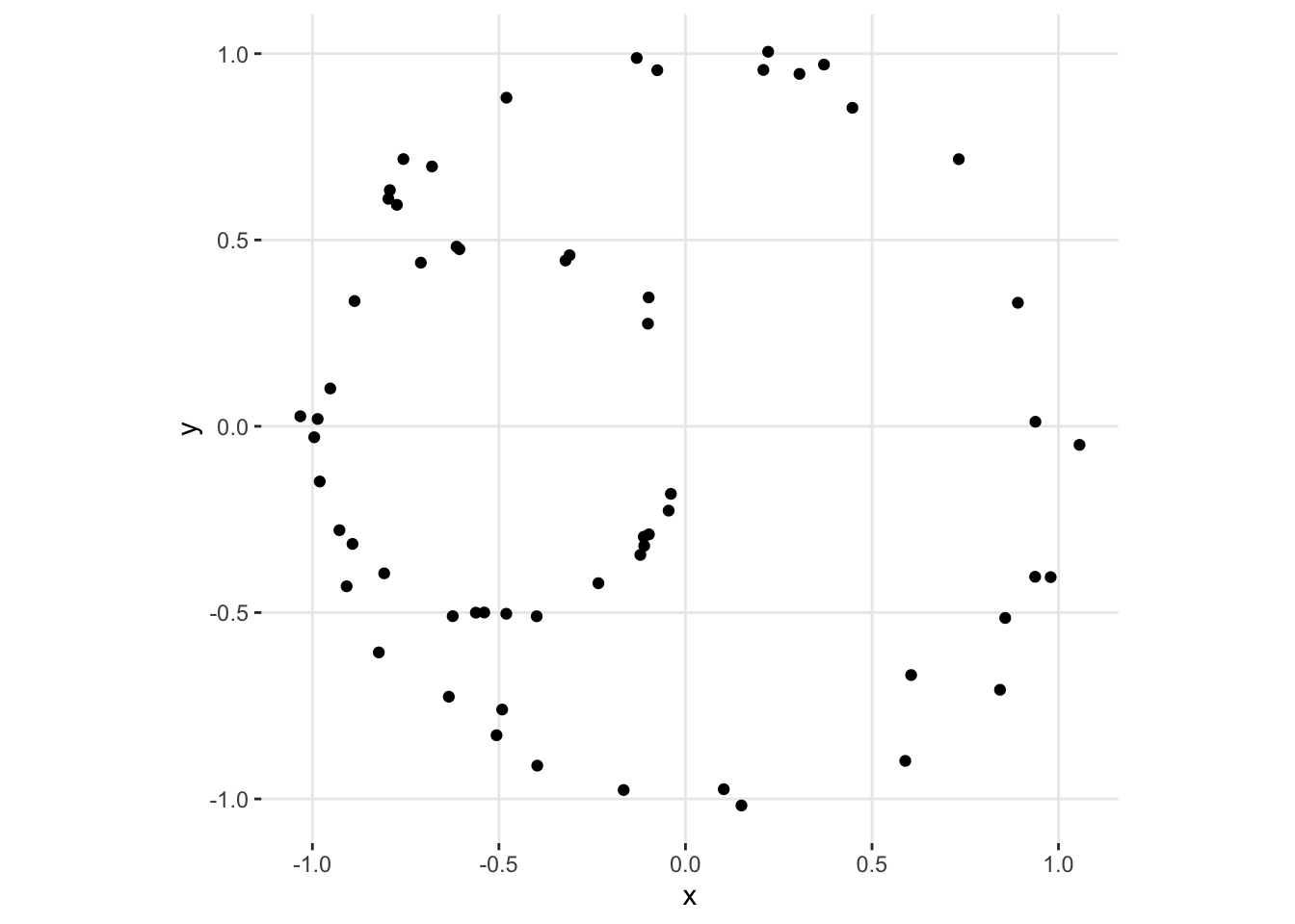
Let’s start with a sample of data in \(\mathbb{R}^2\):

We can see, pretty easily, that we are sampling from two circles, one larger than the other; but our interest is in reaching the same conclusion examining the data algorithmically. This is more clearly seen with higher dimensional data, that cannot be visualized as easily.

Fundamental Geometric Structures

With data, typically referred to as point clouds, we need a way to represent the geometric structure of the data; simplices and simplicial complexes accomplish this.

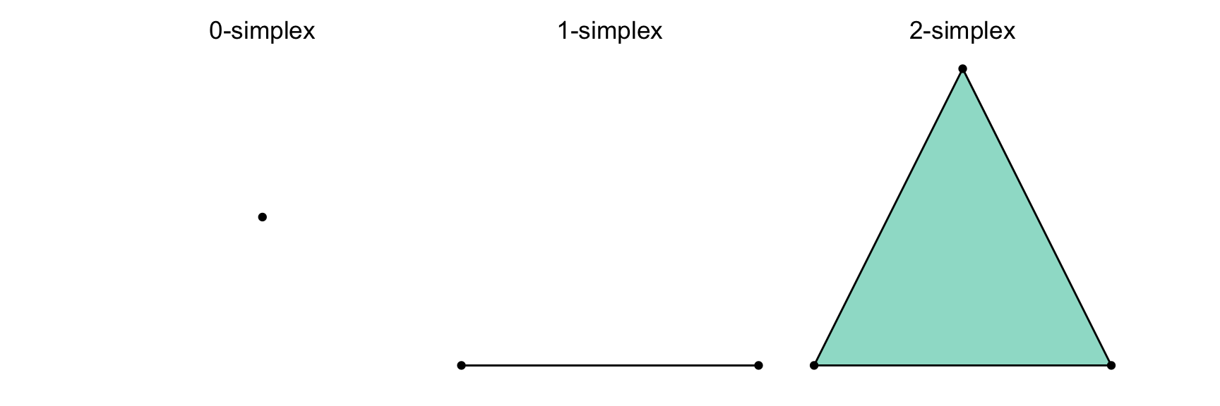
We can think of them like as basic shapes like points, line segments, triangles, tetrahedra.

Formally, a \(k\)-simplex is the convex hull¹ of \(k+1\) geometrically independent points² \(\{v_0, ..., v_k\}\), which we notate as: \([v_0, ..., v_k] = \bigl\{ \sum_{i=0}^k \alpha_i v_i : \sum_{i=0}^k \alpha_i = 1, \alpha_i \ge 0 \bigr\}\).

The 0-simplex, \([v_0]\) , is a point or vertex. The 1-simplex, \([v_0, v_1]\), is a line segment or edge. The 2-simplex, \([v_0, v_1, v_2]\), is a triangle (including its interior). The 3-simplex, \([v_0, v_1, v_2, v_3]\), is a tetrahedron (including its interior). So as we add points, we increase the dimension.

The face of a simplex \(\sigma\) is a simplex formed by removing one or more vertices from \(\sigma\). The convex hull of any nonempty subset of the \(n + 1\) points that define an n-simplex. For example, the faces of a 2-simplex (triangle) are its edges (1-simplices) and vertices (0-simplices).

Simplicial Complexes

Now we need a way to connect or glue the simplices together; these glued structures are called simplicial complexes. For a set of simplices, we can determine if they form a complex if they satisfy two properties: face inclusion and consistent intersection.

If we have a simplicial complex \(S\), then it has face inclusion if a simplex \(\xi \in S\) implies that all faces of \(\xi\) are also in \(S\). It has consistent intersection if for any pair of simplices \(\xi_1, \xi_2 \in S\), their intersection is either empty (\(\emptyset\)) or contained in \(S\). Now we will cover the most common complexes used in TDA: Vietoris-Rips, Čech, Delaunay, and Alpha complexes.

Vietoris-Rips

Vietoris-Rips complexes are a way to build simplicial complexes from point clouds based on proximity.

Given a point cloud \(X = \{x_i\}_{i=1}^L \subset \mathbb{R}^d\), the Vietoris-Rips Complex \(\mathcal{V}_r(X)\) is defined by a proximity radius \(r > 0\) and a rule: a simplex \([x_{i_1}, ..., x_{i_l}] \in \mathcal{V}_r(X)\) iff \(\text{diam} (x_{i_1}, ..., x_{i_l}) \leq r\).

Like all of the complexes we will cover, they are built from points being connected by proximity in euclidean distance. Here if the pairwise distance between points is less than or equal to \(2r\), then they are connected.

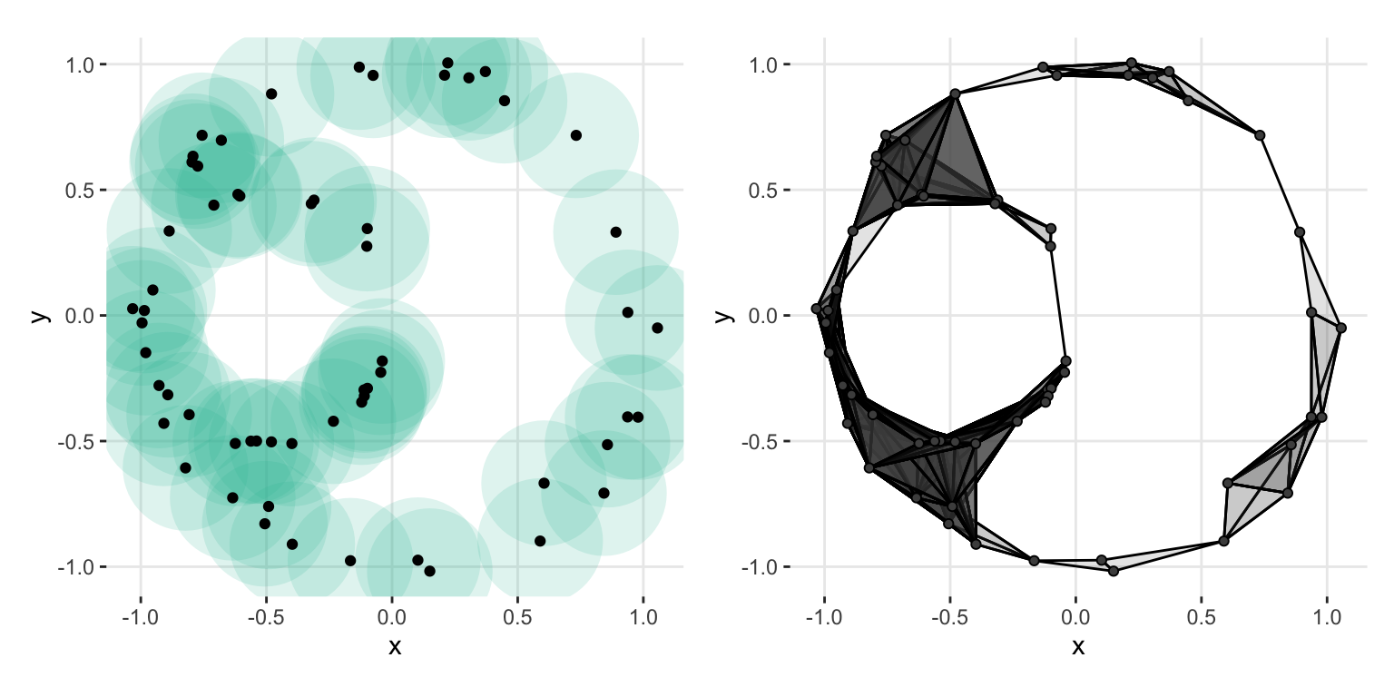
Let’s see what our example data looks like in a Vietoris-Rips complex with a radius of .25. On the left we see the balls³ and their intersections. On the right we see the resulting simplicial complex.

Čech

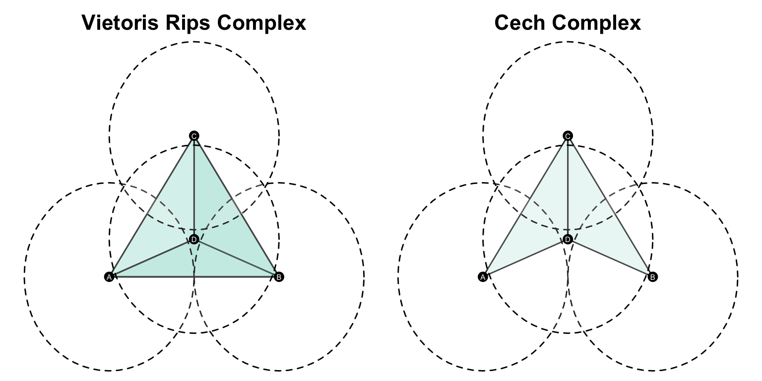
The Čech Complex is similar to the Vietoris-Rips complex, but it uses a different rule for connecting simplices. Instead of connecting points based on pairwise distances, it connects points based on the intersection of all balls of radius \(r\) centered at each point. So between two points, the rule is the same, but for multiple points, it differs.

Formally, \(Čech(r) = \{\sigma \subseteq S | \underset{x \in \sigma}{\bigcap} B_x(r) \neq \emptyset \}\)

If we consider some points, they may all have pairwise distances less than or equal to \(2r\), but the intersection of all the balls may be empty. Here we can see that the Čech complex doesn’t include the simplex containing points \(A, B, C\) because the intersection of the balls together is empty, where the point \(D\) resides. Since the Vietoris-Rips complex connects points based on pairwise distances, it includes the simplex containing \(A, B, C\).

Delaunay & Alpha

The last complexes we will discuss here are the Delaunay and Alpha complexes which are closely related. However, we must first introduce Voronoi cells and diagrams.

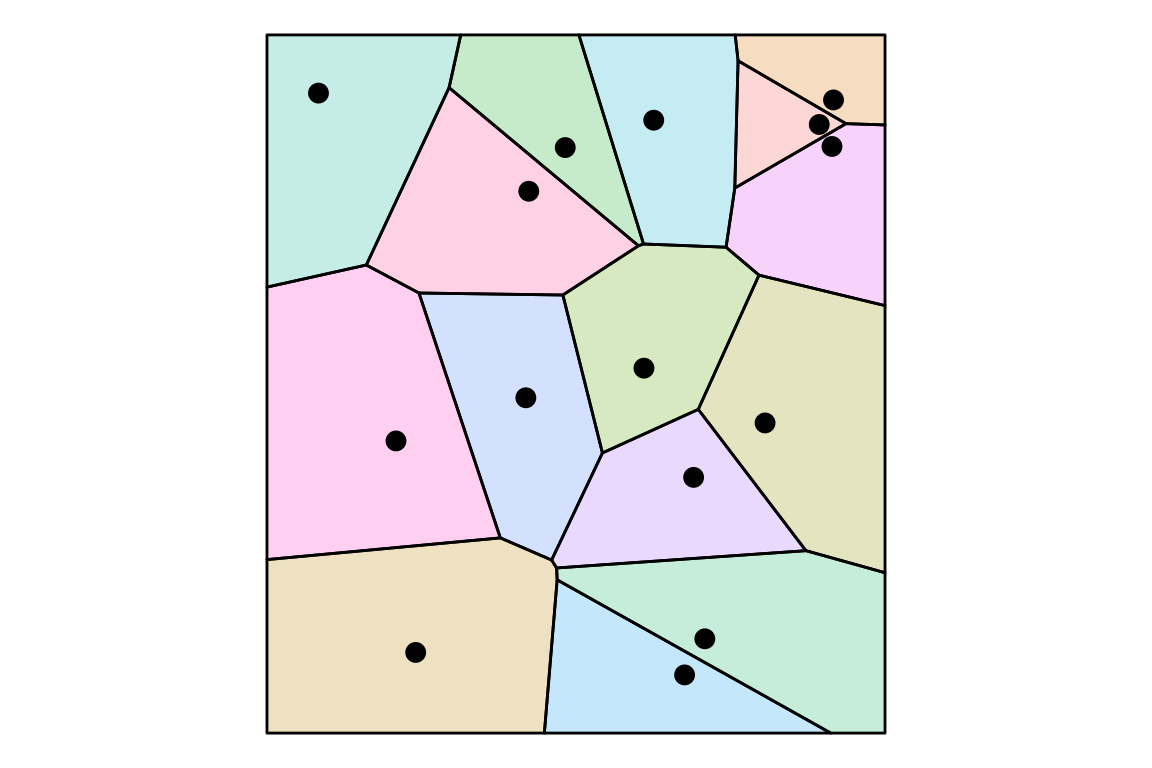
For set of points(sites) in \(S\), a Voronoi Cell (\(V_u\)) is the region of points closer to a site \(u \in S\) than to any other site.

\[ V_u = \{x \in \mathbb{R}^d \mid \|x - u\| \le \|x - v\|, \forall v \in S\} \]

Here, each inequality \(\|x - u\| \le \|x - v\|\) defines a half-space⁴. The cell \(V_u\) is the intersection of these half-spaces, which guarantees it is always a convex polygon (in 2D). The Voronoi Diagram is the collection of all cells \(\{V_u\}_{u \in S}\), which creates a complete partition⁵ (or tessellation) of the space.

Here is the Voronoi diagram of a sample of 15 points.

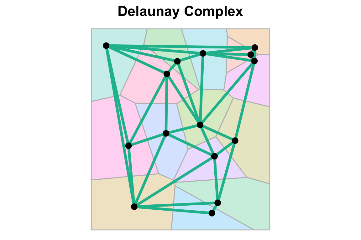
The Delaunay Complex is the dual⁶ of the Voronoi diagram. More formally, it is the nerve of the collection of Voronoi cells.

We create the delaunay complex through a rule: a set of sites \(\sigma \subseteq S\) forms a simplex in the Delaunay complex if and only if their corresponding Voronoi cells have a non-empty intersection:

\[\bigcap_{u \in \sigma} V_u \ne \emptyset\]

This means two sites are connected if their Voronoi cells share an edge and three sites form a triangle if their cells meet at a single vertex. We can see what the Deluanay complex corresponding to the Voronoi diagram we just saw.

To wrap up our discussion over the types of complexes, we have the Alpha complex, which combines the ideas of radii and balls that the Čech and Vietoris-Rips have, with the neighboring cell strucuture the Delaunay has.

The Alpha complex is a subcomplex of the Delaunay complex; it filters the simplices based on a radius, \(r\). A simplex \(\sigma\) is included if the intersection of balls of radius r and their corresponding Voronoi cells are non-empty. The regions are defined by \[R_u(r) = B_u(r) \cap V_u \text{ for each } u\] As \(r\) increases, more simplices are included, until the Alpha complex becomes the full Delaunay complex.

Lastly, these complexes have a hierarchy, where one is nested or a subcomplex of another. The Alpha is the smallest, then Čech, and lastly Vietoris-Rips. For a radius, \(r\):

\[ \text{Alpha}(r) \subseteq \text{Čech}(r) \subseteq \text{Vietoris-Rips}(r) \]

Filtration

For each of the complexes, the choice of radius can have a significant impact on the resulting complex. In this case, we don’t want to use a single radius, but we can use a sequence of radii to give us a sequence of complexes.

For a nondecreasing sequence \(\{ r_n\} \in \mathbb{R}^+ \cup \{ 0\}\) with \(r_0 = 0\), we denote the filtration by \(\{ \mathcal{C}_{r_n} (X)\}_{ n\in \mathbb{N}}\), for a complex \(\mathcal{C}\).

The filtration is a sequence of nested simplicial complexes; so for Vietoris-Rips complexes, we have:

\[ \mathcal{V}_{r_0}(X) \subseteq \mathcal{V}_{r_1}(X) \subseteq \mathcal{V}_{r_2}(X) \subseteq \dots \]

Note that as we increase the radius \(r\), more points get connected, and higher-dimensional simplices appear. This filtration tracks how the structure, holes and voids, changes as the scale of \(r\) changes. This is what the Vietoris Rips filtration of our data would look like.

From here, we can use these sequences of complexes to identify features/shapes/holes in the data, which will be discussed next.

Interactive Vietoris-Rips Visualization

An interactive shiny app to visualize the Vietoris-Rips filtration of a point cloud is available here.

Navigation

To go back to the listings, click here. To view the next article on Homology, click here.

Footnotes

1. The convex hull of a set of points is the smallest convex set(polygon) that contains all the points.

2. Geometrically independent means the points are affinely independent, i.e., no point can be expressed as a linear combination of the others.

3. In Euclidean \(n\)-space, an (open) \(n\)-ball of radius \(r\) and center \(x\) is the set of all points of distance less than \(r\) from \(x\). A closed \(n\)-ball of radius \(r\) is the set of all points of distance less than or equal to \(r\) away from \(x\). See here.

4. The two parts into which a hyperplane divides an n-dimensional space. See here

5. Here partition rfefers to the partition of a set, a grouping of the elements into non-empty subsets, where each element is included in exactly one subset. For more see here.

6. Duality translates concepts or structures in math into other concepts or structures in a one-to-one fashion. Here the one-to-one relationship is between the faces and vertices of each. See here